Seasonal Sales Analysis Workflow for E-Commerce Teams

TL;DR:

Effective seasonal sales analysis requires at least 24 months of clean, segmented transaction data to identify reliable patterns. By applying time-series techniques, businesses can forecast demand, plan inventory, and execute timely marketing strategies. Monitoring key metrics during the season helps teams adapt quickly and reduce stockouts or excess inventory.

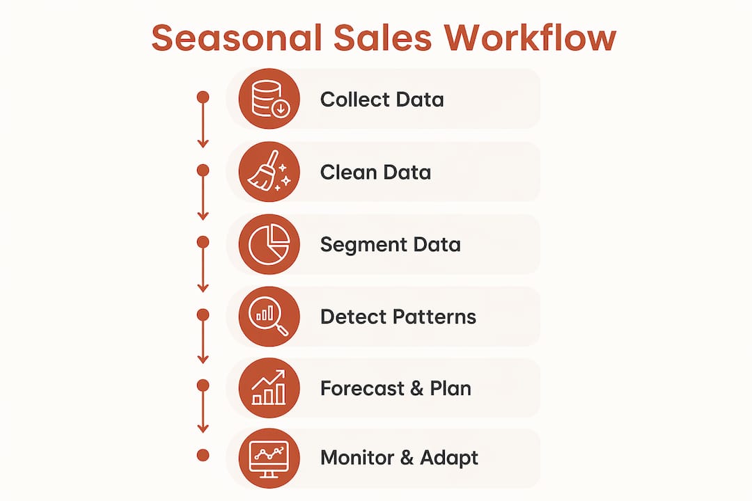
A workflow for analyzing seasonal sales is a structured, repeatable process that turns raw transaction data into accurate demand forecasts, timed inventory orders, and coordinated marketing plans. Most e-commerce teams treat seasonal analysis as a one-time exercise before the holidays. That approach leaves money on the table and creates stockout risk at the worst possible moment. The seasonal sales analysis workflow covered here runs end-to-end: from data collection and cleaning through pattern detection, forecasting, real-time monitoring, and post-season review. Each step builds on the last, so skipping one compounds errors downstream.

What data do you need for a seasonal sales analysis workflow?

The foundation of any seasonal analysis is historical transaction data, and the minimum threshold is clear. You need at least 12–24 months of sales history to identify a repeating seasonal cycle, with 36 months being the standard for reliable pattern detection. Two years of data lets you spot a peak. Three years lets you confirm it is a pattern and not a coincidence.

The specific fields you need in your dataset include:

Order date (day-level granularity, not just month)
SKU or product ID with category and subcategory labels
Units sold and revenue per transaction
Returns and cancellations (net sales, not gross)
Sales channel (direct, marketplace, wholesale)
Geographic region or shipping destination

Once you have the raw data, cleaning it is not optional. Normalize your data by flagging and removing one-time anomalies before you run any analysis. A viral TikTok moment in march 2024 that tripled your candle sales is not a seasonal signal. It is noise. If you leave it in, your forecast will overestimate demand for that same week next year, and you will overstock.

Segment the cleaned data by product category, sales channel, and geographic region before you look for patterns. Seasonality in the American Southwest looks different from seasonality in the Pacific Northwest. A single blended view hides those differences and produces forecasts that are wrong for every segment.

Pro Tip: Export your order data from Shopify, WooCommerce, BigCommerce, or Stripe as a CSV and run your cleaning pass in a spreadsheet before importing into any analytics platform. Catching errors at the source saves hours of rework later.

How do you identify seasonal patterns in your sales data?

Pattern detection is where the seasonal sales analysis process moves from data management to actual insight. Three time-series techniques cover most e-commerce use cases: moving averages, Holt-Winters exponential smoothing, and SARIMA (Seasonal Autoregressive Integrated Moving Average). Each works differently, but all three separate the seasonal component from the underlying growth trend.

The practical starting point for most analysts is the seasonality index. Calculate it by dividing each month’s average sales by the overall average monthly sales across your full dataset. A value above 1.0 means that month outperforms the annual average. A value below 1.0 means it underperforms. Run this calculation for each of your product categories separately, because a single store-level index masks category-level variation.

Avoid confusing long-term growth trends with seasonality by examining your raw time series before applying any smoothing. If your store grew 40% year over year, a naive comparison of this october to last october will show a spike that looks seasonal but is actually just growth. Strip out the trend component first, then look at what remains.

Confirm any pattern you find with at least two repeating cycles. One peak does not make a season. Two peaks in the same calendar window, across two separate years, is the minimum evidence for a reliable seasonal signal.

External data strengthens internal findings. Google Trends lets you cross-reference your sales peaks against broader market search behavior. If your internal data shows a spike in outdoor furniture sales every april, and Google Trends confirms a national search surge for the same category in the same window, you have corroborating evidence that the pattern is real and market-driven, not just an artifact of your own promotions.

Seasonality patterns vary by geographic region, so segment your analysis accordingly. A product that peaks in july in Florida may peak in september in Minnesota. Blending those markets into one forecast produces a number that is wrong for both.

Pro Tip: Use a simple four-column table in a spreadsheet: month, average sales, overall monthly average, and the resulting index. This gives you a seasonality profile you can paste directly into your forecasting model without any specialized software.

How does seasonal analysis translate into forecasting and inventory planning?

Identifying a seasonal pattern is only useful if you act on it before the season starts. The standard pre-season planning timeline begins 12 weeks before your peak, with defined milestones for each phase.

A typical 12-week countdown looks like this:

Weeks 12–10: Complete inventory audit, finalize last season’s sell-through data, and set category-level sales targets.
Weeks 9–7: Run your seasonality index calculations, apply growth rate adjustments, and build your initial demand forecast.
Weeks 6–5: Finalize purchase orders. Domestic suppliers need 3 months lead time; overseas suppliers need 6 months, so international orders must go out well before this window.
Weeks 4–3: Confirm inbound shipment schedules, brief your warehouse team, and align your marketing calendar with confirmed stock arrival dates.
Weeks 2–1: Conduct a final stock check, activate promotional assets, and brief customer service on expected volume increases.

Inventory buffers are not guesswork. Apply a safety stock calculation that accounts for peak-to-trough demand variability, not just average weekly sales. A product that sells 50 units per week in the off-season but 300 units per week at peak needs a safety buffer sized for the peak, not the average.

Staffing is part of the forecast too. Peak season staffing requires planning for additional full-time equivalents based on incremental units sold, covering warehouse picking, packing, and customer service. Treat headcount as a variable in your capacity plan, not an afterthought.

Pro Tip: Build your marketing calendar in the same spreadsheet as your inventory plan. When a promotion goes live before stock arrives, you create demand you cannot fulfill. Aligning both plans in one view makes the conflict visible before it becomes a crisis.

How do you monitor seasonal performance and adapt in real time?

Tracking the right metrics during the season separates teams that react in time from teams that discover problems after the peak has passed. A focused KPI set prevents analysis paralysis and keeps weekly check-ins fast and useful.

The core KPIs for in-season monitoring are:

Daily sales velocity: Units sold per day versus the forecast. A consistent gap of 15% or more in either direction signals a need to act.
Weekly sell-through rate: Percentage of available inventory sold in a given week. A rate that falls behind plan early in the season predicts excess stock at the end.
Promotional uplift: Revenue increase attributable to a specific promotion, net of any cannibalization from other SKUs.
Margin impact: Gross margin per unit, tracked weekly to catch early signs of discount pressure.

When daily velocity runs ahead of forecast, the response options are stock reallocation from slower-moving locations, expedited replenishment, or air freight for fast movers. Each option has a cost. The decision depends on how much margin the product carries and how many selling days remain.

Starting seasonal planning too late and holding stock too long after demand declines are the two most common and costly mistakes in seasonal retail. An exit strategy for leftover inventory should be part of your plan before the season starts, not improvised after it ends. Set a markdown trigger date, typically two to three weeks before the seasonal demand curve drops, and execute it on schedule.

After the season closes, document your forecast accuracy using MAPE (Mean Absolute Percentage Error). MAPE values under 30% indicate a reliable seasonal forecast for e-commerce. If your MAPE exceeds that threshold, trace the error back to a specific step: data quality, pattern detection, or the growth rate assumption. Fix the root cause before next season.

For a deeper look at which e-commerce KPIs matter most for seasonal evaluation, the Affinsy blog covers the full metric set with practical benchmarks. Understanding sales trend patterns across your catalog also helps you distinguish seasonal signals from structural shifts in demand.

Key Takeaways

A reliable seasonal sales analysis workflow requires at least 24 months of clean, segmented transaction data, a confirmed repeating pattern, and a procurement timeline that starts 12 weeks before peak.

Point	Details
Data depth matters	Pull 24–36 months of historical sales data to confirm true seasonal cycles, not one-off spikes.
Clean before you analyze	Remove anomalies and viral events from your dataset before calculating any seasonality index.
Start procurement early	Domestic orders need 3 months lead time; overseas orders need 6 months before your peak date.
Monitor a short KPI list	Track daily velocity, sell-through rate, and margin weekly to catch deviations before they compound.
Plan your exit in advance	Set a markdown trigger date before the season starts to avoid holding excess stock after demand drops.

Why most seasonal analysis fails at the edges of the curve

The part of seasonal analysis that trips up even experienced analysts is not the peak. The peak is obvious. The problems live at the edges: the ramp-up weeks before demand accelerates and the decline weeks after it crests.

I have seen teams nail their peak-week forecast and still end the season with a margin problem because they held full-price inventory two weeks too long. The sell-through data was telling them to mark down. The instinct to “wait one more week” overrode the signal. That is not an analytics failure. It is a process failure. The exit strategy was not written down, so it was negotiable under pressure.

The other edge problem is starting the analysis too late. If you begin your seasonal sales data workflow in october for a holiday peak, your overseas purchase orders are already six weeks late. The analysis was fast. The procurement window was already closed.

The fix for both problems is the same: treat the exit date and the order date as hard constraints in your plan, not estimates. Write them down before the season starts. Attach them to a calendar. Make them non-negotiable. The analysis informs those dates. It does not replace the discipline of honoring them.

One more thing worth saying: trend data from Google Trends or keyword research tools is not a replacement for your own transaction history. It is a sanity check. If your internal data says demand peaks in april and Google Trends says the market peaks in june, that gap deserves investigation before you commit to a forecast. Sometimes your customers are early adopters. Sometimes your data has a problem. Either way, the discrepancy is a signal worth following.

— Mateusz

How Affinsy supports your seasonal analysis process

Seasonal analysis produces the most value when it connects directly to customer behavior, not just product volume. Affinsy analyzes historical transaction data to surface product association patterns and customer segmentation signals that pure sales volume reports miss entirely.

During peak seasons, understanding which products customers buy together, through market basket analysis, lets you build bundles and cross-sell sequences that lift average order value without adding inventory risk. Affinsy connects via CSV upload, API, or MCP, so you can feed it the same cleaned order export you already use for your seasonal forecasting. The permanent free tier covers up to 20,000 line items with no credit card required, making it practical to test on a single season’s data before committing. Pro plans start at $49/month for larger datasets and API access. For teams that want to go deeper on customer segmentation during seasonal campaigns, Affinsy’s RFM analysis identifies which customer groups drive peak revenue and which ones churn after the season ends.

FAQ

How much historical data do I need for seasonal analysis?

Pull a minimum of 12–24 months of sales data to identify a seasonal cycle, with 36 months being the standard for reliable pattern confirmation. Two years catches a peak; three years confirms it repeats.

What is a seasonality index and how do I calculate it?

A seasonality index is each month’s average sales divided by the overall average monthly sales across your full dataset. Values above 1.0 indicate above-average months; values below 1.0 indicate below-average months.

How early should I place purchase orders for a seasonal peak?

Work backward from your peak start date. Domestic suppliers need 3 months lead time; overseas suppliers need 6 months. A 12-week pre-season planning timeline covers both if you start on schedule.

What KPIs should I track during the season?

Track daily sales velocity, weekly sell-through rate, promotional uplift, and gross margin impact. A focused set of four to five KPIs prevents analysis paralysis and keeps weekly reviews fast and decision-ready.

How do I measure forecast accuracy after the season?

Calculate MAPE (Mean Absolute Percentage Error) by comparing your forecasted units to actual units sold. A MAPE under 30% indicates a reliable seasonal forecast for e-commerce. Values above that threshold point to a specific step in your workflow that needs correction.